Module/guidance vector field

Modules

ArduIMU

Module/ADC generic

Module/Aeroprobe OTF

Module/Airspeed ETS

Module/AOA adc

Module/Bosch BMP085

Module/collective tracking control

Module/FlightBenchmark

Module/Freescale MPL3115A2

Module/GPS UBlox UCenter

Module/guidance vector field

Module/Honeywell HIH-4030

Module/Hygrosens TEMOD-I2C-R1

Module/infrared

Module/IST DigiPicco

Module/LM75

Module/Mag HMC58xx

Module/Meas Spec MS5611 I2C

Module/Melexis MLX90614

Module/rl obstacle avoidance

Module/Rotorcraft cam

Module/Sensirion SHT25

Module/Sensirion SHT75

Module/Servo switch

Module/System monitor

Module/TI TMP102

Module/TronSens HTM B71

Module/VTI SCP1000 I2C

Module/VTI SCP1000 SPI

Modules

Modules list

MultiUAV

Openlog

Pan Tilt Camera

SDLogger SPI Direct

Sensors/AMSYS

Introduction

We have written an algorithm for solving the problem of tracking smooth curves by an unmanned aerial vehicle travelling with a constant airspeed and under a wind disturbance. The algorithm is based on the idea of following a guiding vector field which is constructed from the implicit function that describes the desired (possibly time-varying) trajectory.

For fixed-wings the output of the algorithm can be directly expressed in terms of the bank angle of the UAV in order to achieve coordinated turns. Furthermore, the algorithm can be tuned offline such that physical constraints of the UAV, e.g., the maximum bank angle, will not be violated in a neighborhood of the desired trajectory.

The implementation for rotorcraft is still in the TO DO list.

This work is based on the paper Guidance algorithm for smooth trajectory tracking of a fixed wing UAV flying in wind flows, presented at ICRA 2017. A more rigorous and detailed analysis can be found in the paper A guiding vector field algorithm for path following control of nonholonomic mobile robots.

We can further exploit the convergence properties of the fixed-wing aircraft to the desired trajectory for controlling formations of several aircraft. Check the subsection python Apps. A detailed analysis can be found in the paper Circular formation control of fixed-wing UAVs with constant speeds (submitted to IROS 2017). A video about how the circular formation algorithm works https://www.youtube.com/watch?v=q4b8JRU1Gbw .

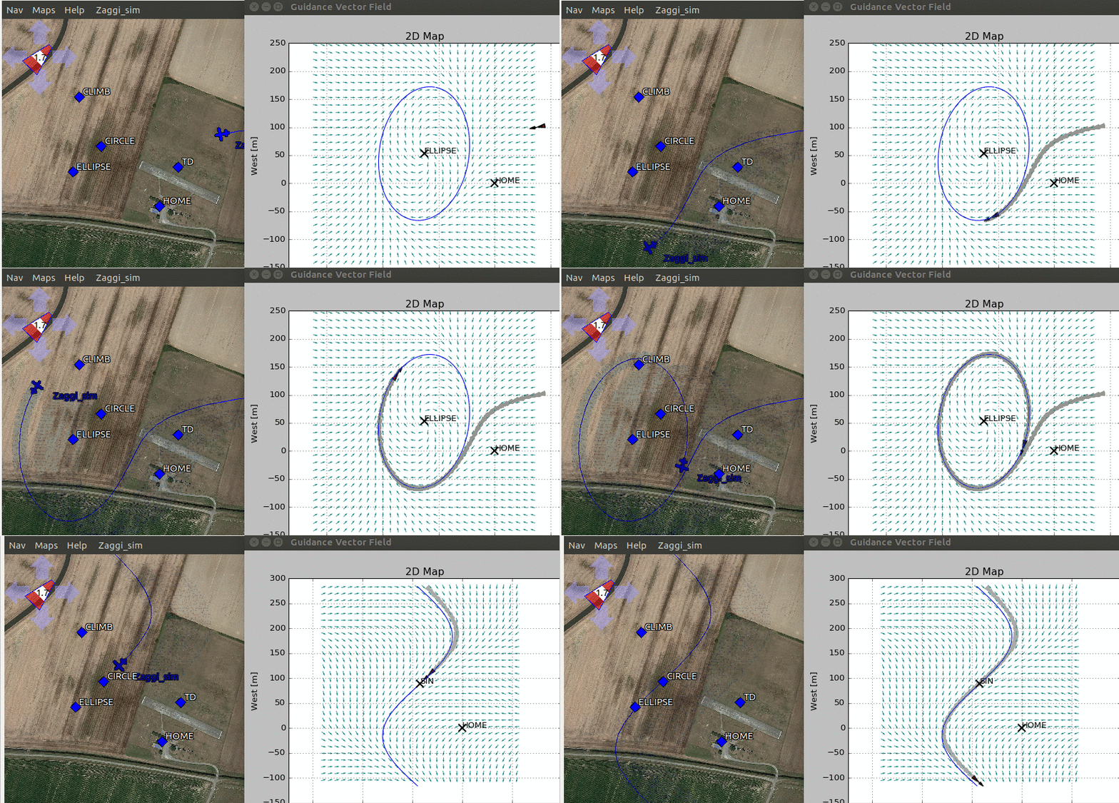
Here we show an animation of an airplane following an ellipse and a sinudoidal track.

How does the algorithm work?

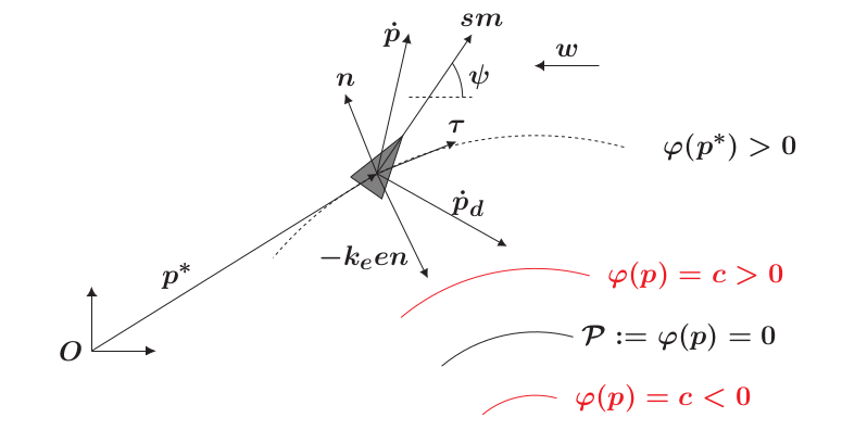
We start from the implicit equation of the trajectory, for example for a circumference we have that $\varphi (x,y)=x^{2}+y^{2}-R^{2}$, where $x,y$ and $R$ are the x, y coordinates with respect to HOME ($O$ in the following figure) and R is the radius of the circumference. Note that when the vehicle is over the desired trajectory, then $\varphi (x,y)=0$, otherwise it will be different from zero. We will use this concept of "level set" to define the notion of distance to the trajectory, namely $e:=\varphi (x,y)$. It has to be noted that this is different from the Euclidean distance (see figure below).

For the sake of clarity we will consider just 2D trajectories and parallel to the ground. Let us stack the x and y coordinates in $p:={\begin{bmatrix}x&y\end{bmatrix}}^{T}$ and consider the following kinematical model for our vehicle

${\begin{cases}{\dot {p}}&=sm(\psi )+w\\{\dot {\psi }}&=u,\end{cases}}$

where $s\in \mathbb {R} ^{+}$ is a constant that can be considered as the airspeed, $m={\begin{bmatrix}\cos(\psi )&\sin(\psi )\end{bmatrix}}^{T}$ with $\psi \in (-\pi ,\pi ]$ being the attitude yaw angle, $w\in \mathbb {R} ^{2}$ is a constant with respect to $O$ representing the wind and $u$ is the control action that will make the vehicle to turn. We also notice that the course heading $\chi \in (-\pi ,\pi ]$, i.e. the direction the velocity vector ${\dot {p}}$ is pointing at, in general is different from the yaw angle $\psi$ because of the wind.

Given a desired trajectory, we compute its normal $n(p):=\nabla \varphi (p)$ and its tangent $\tau (p)=En(p),\quad E={\begin{bmatrix}0&1\\-1&0\end{bmatrix}}$. The idea is to steer the vehicle such that it follows the direction given by the unit vector calculated from

${\dot {p}}_{d}(p):=\tau (p)-k_{e}e(p)n(p),$

where $k_{e}$ is a positive gain. At each point $p$ we can build a unit vector from ${\dot {p}}_{d}(p)$. This collection of vectors is our Guidance Vector Field. Note that when the error is zero, then we are just tracking the tangent to the trajectory.

We assume that the trajectory is twice differentiable (so its gradient and Hessian exists) and that it is regular in a neighborhood of ${\mathcal {P}}$, i.e.

$\nabla \varphi (p)\neq 0,\quad p\in {\mathcal {N}}_{\mathcal {P}},\quad {\mathcal {N}}_{\mathcal {P}}:=\{p\,:\,|\varphi (p)|\leq c^{*}>0\}$.

The algorithm needs for work the measurements of ${\dot {p}}$ (typically derived from GPS), position $p$ w.r.t. HOME (typically derived from GPS) and yaw angle $\psi$ or sideslip angle $\beta =(\psi -\chi )$. The algorithm still works quite well in practice with only ${\dot {p}}$ and $p$, in other words, you will only need to have installed a GPS. The latter is the implemented version in pprz/master.

Using the GVF in the flight plan

{TODO: to enumerate all the functions available for the user.}

So far we have added support for two kind of trajectories, ellipses and sinusoidals. Note that the former includes circumferences and the latter includes straight lines (zero frequency).

For tracking an ellipse, one has to call the function

<call fun="gvf_ellipse(WP_STDBY, gvf_ellipse_a, gvf_ellipse_b, gvf_ellipse_alpha)"/>

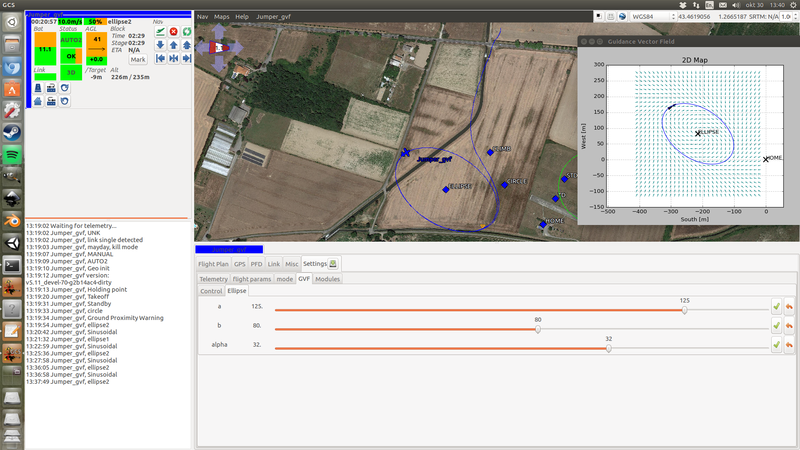
where gvf_ellipse_a (horizontal axis), gvf_ellipse_b (vertical axis), gvf_ellipse_alpha (rotation w.r.t. North) can be defined in your settings file.

For tracking a straight line that crosses HOME with course heading 45 degrees

<call fun="gvf_line_wp_heading(WP_HOME, 45)"/>

For tracking a sinusoidal, the same as the straight line but including the additional information about frequency, offset and amplitude (in meters)

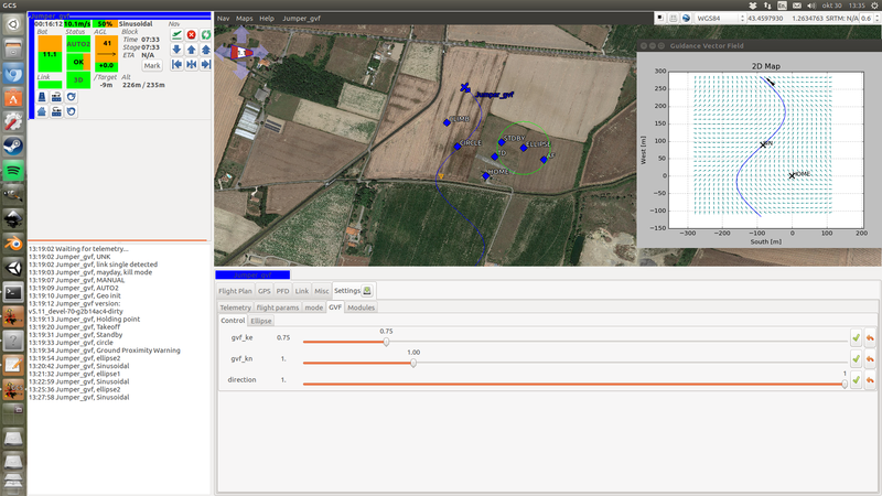
<call fun="gvf_sin_wp_heading(WP_HOME, course_heading, freq, off_set, amplitude)"/>

For setting the tracking direction (the direction of the tangent vector $\tau$ in the above figure)

<call fun="gvf_set_direction(s)"/>

where s is an integer number 1 or -1.

Gain tuning

The user has to tune two gains $k_{n},k_{e}$. The former one determines the convergence rate for aligning the vehicle to the vector field. A typical value for starting tuning $k_{n}$ should be between 0.2 and 1. The latter gain determines how aggressive is the vector field. For example, in the following figure we have an ellipse with two different values of $k_{e}$, at the left we have a value of 3 and at the right 0.4. Note how in left one the vectors are "more aggressive" towards the trajectory. While a big value can make the vehicle to converge quickly to the trajectory, it can make the tracking unstable once the vehicle is close it. This is because the vector field might change so quick that physically the vehicle cannot follow it. Check the Section IV in the original paper in the introduction.

It is a good practice in the flight plan to set the gains before calling the trajectory since it is pretty common to have different gains for different trajectories. For example

<call fun="gvf_set_direction(s)"/>
<call fun="gvf_set_gains(ke, kn)"/>
<call fun="gvf_ellipse(WP_STDBY, gvf_ellipse_a, gvf_ellipse_b, gvf_ellipse_alpha)"/>

Python Apps

Visualizing the desired trajectory and the aircraft within the vector field

Until the "visual integration" of the GVF into the ground station is ready, one can track the vehicle and the trajectory by using the python script at "$PAPARAZZI_HOME/sw/ground_segment/python/gvf/gvfApp ac_id", where ac_id is the ID of the fixedwing to be tracked by the App.

• 
• 

Circular formations

One can synchronize or arrange a group of fixed-wing aircraft (assuming they have equal ground speed) in a desired circle by using the python script at "$PAPARAZZI_HOME/sw/ground_segment/python/gvf/gvfFormation". For running the script, all your aircraft MUST follow a circle employing the guidance vector field, i.e.,

<call fun="gvf_ellipse(WP_STDBY, gvf_ellipse_a, gvf_ellipse_b, gvf_ellipse_alpha)"/>

the values of gvf_ellipse_a, gvf_ellipse_b will be modified by the formation control script, and the value of gvf_ellipse_alpha is irrelevant. Note that the aircraft do not need necessarily to orbit around the same waypoint.

We need three text files in order to run the script:

• ids.txt , which labels the aircrafts. For example, if the file contains '14 56 34', then the aircraft with ids 14, 56 and 34 are labeled with the tags 1, 2 and 3 respectively.
• topology.txt , which defines the links between the aircraft. The file contains a matrix where the number of rows is the number of aircraft, and the number of columns is the number of desired links. A link is defined by setting 1 and -1 in a column. Following the example, the matrix ${\begin{bmatrix}1&0\\-1&1\\0&-1\end{bmatrix}}$ defines two links. The first one between the aircraft 1 and 2, and the second one between the aircraft 2 and 3.
• sigmas.txt , which defines the desired angles $\sigma _{k}$ between aircraft for each link $k$. Following the example, if the file contains '0 90', then the desired angle for the first link is 0 degrees (e.g., the aircraft 1 and 2 will meet each other) and the second desired angle will be +90 degrees (positive is clock-wise).

Some useful tips:

• How you place 1 and -1 in the topology matters in the following sense. In our example, for the second link, the +90 degrees is from the aircraft 2 to the aircraft 3. If the topology were ${\begin{bmatrix}1&0\\-1&-1\\0&1\end{bmatrix}}$, then the +90 degrees will be from the aircraft 3 to the aircraft 2.
• Watch out for "impossible" configurations, e.g., do not set up loops in the topology such as 1 -> 2 -> 3 -> 1 ${\begin{bmatrix}1&0&-1\\-1&1&0\\0&-1&1\end{bmatrix}}$, so the desired sigmas could be asking for an impossible configuration in the circle. Avoid loops! even if the desired configuration is ok, they can introduce undesired equilibria in the system, i.e., different configurations.
• The aircraft do not need to share the same center or waypoint. This script just control the sigmas.

The script needs two additional scalar values:

• radius , sets the desired radius of the circular formation, i.e., once the aircraft are synchronized, they will be orbiting the waypoint with this desired radius.
• k, this is the gain of the control algorithm. As an example, for three aircraft with a desired circumference of 80 meters, a value of $k=10$ works ok.

The algorithm works by setting different radii to the aircraft. If two aircraft orbit a waypoint with different radius (assuming equal ground speeds), then the one with bigger radius travels more distance in a completed lap. We exploit this fact in order to control the different $\sigma _{k}$. We refer to Circular formation control of fixed-wing UAVs with constant speeds for details about the control signal and how to calculate an appropriated gain k.

In the following figure we show the rendezvous of three aircraft in the same circle by using this script.

Defining your own trajectory

The algorithm is placed in $PAPARAZZI_HOME/sw/airborne/modules/guidance/gvf . The trajectories are placed in $PAPARAZZI_HOME/sw/airborne/modules/guidance/gvf/trajectories .

Here there is an example (the straight line) about how to code your own trajectory. You need to add at least two functions in the header

File:

sw/airborne/modules/guidance/gvf/gvf.h // Straigh line void gvf_line(float x, float y, float alpha); extern bool gvf_line_wp1_wp2(uint8_t wp1, uint8_t wp2); extern bool gvf_line_wp_heading(uint8_t wp, float alpha);

where the first function will be called by the algorithm and the rest by the user in the flight plan. For example, the user in the flight plan calls to gvf_line_wp_heading

File:

sw/airborne/modules/guidance/gvf/gvf.c bool gvf_line_wp_heading(uint8_t wp, float alpha) { alpha = alpha*M_PI/180; float a = waypoints[wp].x; float b = waypoints[wp].y; gvf_line(a, b, alpha); return true; }

The idea is that while you can define a straight line in many different ways, you make all the transformations in the function called by the user such that the algorithm is always evaluating the trajectory in the same way. It helps for maintaining the code and for tuning the gains (you do not want to have different set of gains depending on how you call your trajectory).

We finally call the function gvf_line (hidden for the user) that will invoke the algorithm.

File:

sw/airborne/modules/guidance/gvf/gvf.c void gvf_line(float a, float b, float alpha) { float e; struct gvf_grad grad_line; struct gvf_Hess Hess_line; gvf_traj_type = 0; gvf_param[0] = a; gvf_param[1] = b; gvf_param[2] = alpha; gvf_line_info(&e, &grad_line, &Hess_line); gvf_control_2D(1e-2*gvf_ke, gvf_kn, e, &grad_line, &Hess_line); gvf_error = e; }

The three first lines are the $\varphi (p),\nabla \varphi (p)$ and $H(\varphi (p))$, where $H$ stands for the Hessian. These three guys will be populated by gvf_line_info (in a moment we will be see how to write it).

Then gvf_traj_type stands for the kind of trajectory. Right now we have 0 for lines, 1 for ellipses and 2 for sinusoidals. Feel free to choose an index that has not been taken. The rest gvf_param[x]'s are the parameters of the trajectory. You have up to seven for describing a trajectory.

The function gvf_control_2D executes the algorithm for calculating the desired turn for the vehicle. It is a good practice that all the trajectories (not only straight lines) have the same order of magnitude (between 0.00 and 5.00) for $k_{e}$. So if you have to add a scaling factor, here is were you have to do it.

The variables gvf_xx are sent to the ground station as telemetry, so you can draw the vector field, the trajectory, etc.

Finally for defining $\varphi (p),\nabla \varphi (p)$ and $H(\varphi (p))$ you need to write the two files gvf_line.{c,h}

File:

sw/airborne/modules/guidance/gvf/trajectories/gvf_line.h extern void gvf_line_info(float *phi, struct gvf_grad *, struct gvf_Hess *);

and in gvf_line.c you write the implicit math of your trajectory (quite explicit)

File:

sw/airborne/modules/guidance/gvf/trajectories/gvf_line.c void gvf_line_info(float *phi, struct gvf_grad *grad, struct gvf_Hess *hess){ struct EnuCoor_f *p = stateGetPositionEnu_f(); float px = p->x; float py = p->y; float a = gvf_param[0]; float b = gvf_param[1]; float alpha = gvf_param[2]; // Phi(x,y) *phi = -(px-a)*cosf(alpha) + (py-b)*sinf(alpha); // grad Phi grad->nx = -cosf(alpha); grad->ny = sinf(alpha); // Hessian Phi hess->H11 = 0; hess->H12 = 0; hess->H21 = 0; hess->H22 = 0; }

I have omitted it, but of course you have to take care of all the headings files and to add your new trajectory in $PAPARAZZI_HOME/conf/modules/gvf_module.xml

Demo

There is a flightplan called 'demo_gvf.xml' in order to test the different settings in a simulation. Do not forget to choose default_telemetry_gvf.xml in your paparazzi center.

TO DO list

• Better integration of the GVF with the ground station
• Support to rotorcrafts