Actuator Dynamics

An RPM sensor

A Saleae logic analyzer

A screenshot from the Saleae logic analyser software

An example of estimated actuator dynamics in Matlab

Some stabilization modules require an estimation of the current actuator states. Examples are the INDI and INCA modules. When actuator feedback is not available, this estimation can be mathematical model of the actuators. For brushless motors, a first order transfer function often suffices as actuator model. This guide describes how to accurately determine a first order approximation for a motor with a propeller. Note that the actuator dynamics vary for each configuration of different motors, propellers and ESCs (Electronic Speed Controllers). Used for this example are:

• Cobra C-2814/16 brushless motor, KV=1050
• HQProp 7040 7x4 Propeller Slow Flyer 2 Blade Nylon/Glass Fiber Composite
• KISS ESC 24A re – 32bit Electronic Speed Controller
  
  

Actuator model

With this method, actuators are approximated by a first order model in de following form:

$H_{act}={\frac {K}{\tau s+1}}$

where $H_{act}$ is the actuator transfer function in the Laplace domain, $K$ is the system's gain, and $\tau$ is the system's time constant.

When using such a model on discrete time systems, an estimation of an actuator's current position ($\delta _{est}$) can be calculated as a function of the current actuator command ($\delta$) and the previous estimation of its position ($\delta _{prev}$):

$\delta _{est}=\delta _{prev}+\alpha (\delta -\delta _{prev})$
where $\alpha =1-e^{-\tau \Delta t}$
where $\Delta t$ is the duration of one time step

To make a good approximation of actuator dynamics, one needs to determine appropriate values for $\tau$ and $\alpha$

Measuring Actuator Response

The first step in approximating actuator dynamics is to measure actuator response. This can be done with by connecting an RPM sensor to the motor's wires, and recording both the ESC's input PWM and output RPM signals. An schematic representation of the setup used for this example is shown in the figure below:

Used for the setup of this example:

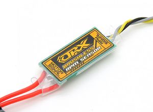
• Orange RPM Sensor for RPM measurements
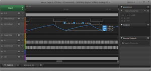
• Saleae Logic 8 for recording measurements
• MATLAB for analyzing measurements
  
  

WORK IN PROGRESS

%{
This script is written for estimation of first order actuator dynamics for
motors with rotors. It uses measurements of both a PWM input signal and the
actuator's RPM response, and tries to fit a first order model to these data
of de form:

     K     
-----------
tau * s + 1

This form can be used to estimate a actuator's state as a function of its
previous state and its current input as follows:

u_est = u_prev + alpha * (u - u_prev)
where alpha = 1 - e^(tau * dt)

© H.J. Karssies - Delft University of Technology
%}

% Close figures and clear workspace
clc
clear all
close all

% Settings
data_file = 'motor_data_04.mat';    % Data file
pwm.channel_no = 0;                 % Channel number of PWM input data
pwm.period_min = 0.0005;            % Minimum PWM period used for filtering
rpm.channel_no = 1;                 % Channel number of RPM measurement data
rpm.period_min = 0.00005;           % Minimum RPM period used for filtering
t_min = 5;                          % Starting time of relevant data (s)
t_max = 10.4;                       % End time of relevant data (s)
taus = 5:5:100;                     % List of values for tau to try (s)
main_freq = 512;                    % Paparazzi main frequency

% Load data
raw_data = load(data_file);
pwm = load_channel(pwm, raw_data);
rpm = load_channel(rpm, raw_data);
pwm.freq = length(pwm.time)/(pwm.time(end)-pwm.time(1));

% Calculate motor frequencies
pwm.motor_freq = pwm.period*1000000;
rpm.motor_freq = 1./rpm.period;

% Check performance for different values of tau
for n = 1:length(taus)
    errors(n) = calc_performance(taus(n), pwm, rpm, t_min, t_max, false);
end

% Interpolate results and find minimum
taus_int = taus(1):0.01:taus(end);
errors_int = spline(taus, errors, taus_int);
error_min = min(errors_int);
tau_min = taus_int(find(errors_int == error_min));
alpha = 1-exp(-tau_min/main_freq);

% Plot result
figure;
set(gcf, 'Position',  [100, 100, 1080, 540]);
subplot(1,2,1);
plot(taus_int, errors_int);
hold on
scatter(tau_min, error_min, 'black');
grid on
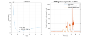
title("\tau estimation");
xlabel("\tau (s)");
ylabel("Error (rpm²)");
text(tau_min, error_min+0.1*diff(ylim), ...
    [sprintf("\\tau = %.2f s", tau_min); ...
    sprintf("\\alpha = %.5f (%d Hz)", [alpha, main_freq])]);

% Perform calculations with final tau and plot figures
calc_performance(tau_min, pwm, rpm, t_min, t_max, true);

% Load channel data and process it
function channel = load_channel(channel, data)
    
    % Process channel
    channel_data = eval('data.digital_channel_' + string(channel.channel_no));
    channel.bit_1 = data.digital_channel_initial_bitstates(channel.channel_no+1);
    channel.period = channel_data(2-channel.bit_1:2:end)./data.digital_sample_rate_hz;
    channel.time = cumsum(channel_data./data.digital_sample_rate_hz);
    channel.time = channel.time(2-channel.bit_1:2:end);

    % Filter out invalid data
    channel.time = channel.time(channel.period>channel.period_min);
    channel.period = channel.period(channel.period>channel.period_min);

end

% Calculate performance with certain tau
function error = calc_performance(tau, pwm, rpm, t_min, t_max, plot_fig)
    
    % Simulate RPM response
    motor = tf(tau,[1 tau]);

    % Run simulation at rounded PWM sample times
    bias = mean(pwm.motor_freq(1:10));
    dt = 1/round(pwm.freq);
    t = [0:length(pwm.time)-1]*dt;
    motor = tf(tau,[1 tau]);
    sim_pwm_freq = lsim(motor, pwm.motor_freq-bias, t) + bias;

    % Get the RPM requency values at the rounden PWM sample times
    int_rpm_freq = interp1(rpm.time,rpm.motor_freq,t,[],1)';
    int_rpm_freq(isinf(int_rpm_freq)) = 1;

    % Fit a simple model y = ax + b
    data_range = and(t>=t_min, t<=t_max);
    inputs = [ones(size(sim_pwm_freq(data_range))) ...
        sim_pwm_freq(data_range)];
    gain = inputs \ int_rpm_freq(data_range);
    sim_rpm_freq = inputs*gain;

    % Calculate squared error
    error = sum((int_rpm_freq(data_range)-sim_rpm_freq).^2);
    
    % Plot figure
    if plot_fig
        subplot(1,2,2);
        plot(pwm.time, pwm.motor_freq)
        hold on
        plot(rpm.time, rpm.motor_freq)
        plot(pwm.time(data_range), sim_rpm_freq)
        grid on
        xlim([0, max(pwm.time)]);
        ylim([0, 1.2*max(rpm.motor_freq)]);
        plot([t_min t_min], ylim, 'black');
        plot([t_max t_max], ylim, 'black');
        title(sprintf("PWM signal and response for \\tau = %.2f s", tau));
        xlabel("Time (s)");
        ylabel("Duty time (ms) / motor speed (rpm)");
        legend(["PWM signal", "RPM measurement", ...
            "Response approximation"])
    end
    
end