RotorcraftMixing

This page describe how to compute "mixing" for an arbitrary multirotors configuration.

Introduction

"Mixing" consist in converting rotational accelerations commands computed by the autopilot into throttle commands for each of the motor controllers.

Let us consider a vehicle comprising a set of $N$ identical fixed pitch rotors $R_{i},i\in [1:N]$ located at coordinates $(X_{i},Y_{i},0),i\in [1:N]$ and spinning in the same plane in the direction $D_{i},i\in [1:N],D_{i}\in [-1;1]$ at a rotational speed $\omega _{i},i\in [1:N]$.

Assuming a quasi hovering regime, the force produced by each rotor can be considered normal to the rotor plane and proportional to the square of its rotational speed. Expressed in body frame ( front, right, down ), this leads to ${\overrightarrow {F}}_{i}^{B}={\begin{pmatrix}0\\0\\-C_{t}\omega _{i}^{2}\end{pmatrix}}$

Under the same assumption, the torque produced by each rotor can also be assumed to be in the same direction and proportional to the square of the rotational speed.

The torque produced by each rotor around the CG, expressed in body frame can then be writen

${\overrightarrow {M}}_{i}^{B}={\begin{pmatrix}X_{i}\\Y_{i}\\0\end{pmatrix}}\wedge {\begin{pmatrix}0\\0\\-C_{t}\omega _{i}^{2}\end{pmatrix}}+{\begin{pmatrix}0\\0\\D_{i}C_{m}\omega _{i}^{2}\end{pmatrix}}$

${\overrightarrow {M}}_{i}^{B}=C_{t}\omega _{i}^{2}{\begin{pmatrix}-Y_{i}\\X_{i}\\D_{i}{\frac {C_{m}}{C_{t}}}\end{pmatrix}}$

Where $C_{t}$ is a "thrust" coefficient and $Cm$ is a "torque" coefficient. It has been measured experimentally that ${\frac {Ct}{Cm}}\approx 10$ on a mikrokopter.

As a first approximation we can consider that the rotational speed of the propeller is proportional to the square root of the applied command $u_{i}$

$\omega _{i}^{2}=Ku_{i}$

This allows us to express the torque produced by the set of rotors as

${\overrightarrow {M}}^{B}=\sum _{i=1}^{N}{\overrightarrow {M}}_{i}^{B}=KC_{t}{\begin{pmatrix}-\sum _{i=1}^{N}Y_{i}u_{i}\\\sum _{i=1}^{N}X_{i}u_{i}\\{\frac {C_{m}}{C_{t}}}\sum _{i=1}^{N}D_{i}u_{i}\end{pmatrix}}$

which can be rewriten as a matrix vector product

${\overrightarrow {M}}^{B}=KC_{t}{\begin{pmatrix}-Y_{1}&-Y_{2}&\ldots &-Y_{n}\\X_{1}&X_{2}&\ldots &X_{n}\\{\frac {C_{m}}{Ct}}D_{1}&{\frac {C_{m}}{Ct}}D_{2}&\ldots &{\frac {C_{m}}{Ct}}D_{n}\end{pmatrix}}{\begin{pmatrix}u_{1}\\u_{2}\\\vdots \\u_{n}\end{pmatrix}}$

${\overrightarrow {M}}^{B}=A{\overrightarrow {U}}$

$A$ is a $3*N$ matrix describing the geometric positions of our rotors and $U$ is the vector of throttle commands for our set of motor controllers.

In order to express the command applied to each power train as a function of the momentum we want to apply to our vehicle, we need to find $B$, a $N*3$ matrix such as

${\overrightarrow {U}}=B{\overrightarrow {M}}^{B}$

If $A$ has rank 3, we know that such a matrix exists (yeah, we can't do 2 rotors or have all rotors aligned), and in this case, we have the relationship

$AB={\mathcal {I}}_{3}$

We know that one solution of this equation is the Moore-Penrose pseudoinverse of $A$. Furthermore, this solution is the one leading to the power train command vector having the smallest euclidian norm, which is interesting as it optimizes the repartion of our control effort across our power trains.

Example

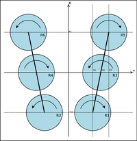
Let's consider the following H hexarotors configuration.

$A={\begin{pmatrix}-0.17&0.17&-0.25&0.25&-0.33&0.33\\-0.35&-0.35&0&0&0.35&0.35\\-0.1&0.1&0.1&-0.1&-0.1&0.1\end{pmatrix}}$

The first two lines of the $A$ matrix represent the coordinates of each rotor in the $X,Y$ plan, and the third line the direction in which they spin.

$B={\begin{pmatrix}-0.24&-0.71&-1.47\\0.241&-0.71&1.47\\-0.93&0.&2.44\\0.93&0.&-2.44\\-0.69&0.71&-1.09\\0.69&0.71&1.09\end{pmatrix}}$

Normalizing columns of $B$ yelds

${\tilde {B}}={\begin{pmatrix}-67&-256&-154\\67&-256&154\\-256&-0&256\\256&0&-256\\-189&256&-115\\189&256&115\\\end{pmatrix}}$

which in turns yelds the following supervision section

   <section name="SUPERVISION" prefix="SUPERVISION_">
    <define name="MIN_MOTOR" value="3"/>
    <define name="MAX_MOTOR" value="200"/>
    <define name="TRIM_A" value="0"/>
    <define name="TRIM_E" value="0"/>
    <define name="TRIM_R" value="0"/>
    <define name="NB_MOTOR" value="6"/>
    <define name="SCALE" value="256"/>
    <define name="ROLL_COEF"   value="{ -67,    67, -256,  256, -189,  189}"/>
    <define name="PITCH_COEF"  value="{ -256, -256,    0,    0,  256,  256}"/>
    <define name="YAW_COEF"    value="{ -154,  154,  256, -256, -115,  115}"/>
    <define name="THRUST_COEF" value="{  256,  256,  256,  256,  256,  256}"/>
  </section>

The above computation can be performed using the following simple octave script

A = [
   0.17   -0.17   0.25  -0.25   0.33   -0.33
  -0.35   -0.35   0.     0.     0.35    0.35
  -0.1     0.1    0.1   -0.1   -0.1     0.1
];

B = pinv(A)

m = max(B)

[nrow,ncol] = size(B)

for i=1:ncol
   Btilde(:,i) = B(:,i)/m(i);
end

Btilde =  round(256*Btilde)